Purpose

This post seeks to explore how Greenville, SC and surrounding areas voted in the 2016 election. It also demonstrates how to retrieve data from the Data.World site. To retrieve data from this site using the tools in this post, you have to create an account (easy to do if you have a Facebook, Twitter, or Github account). You can then get your own API key from your profile page. Furthermore, from R, you will need to get the data.world package (install.packages("data.world")). You can then load the API key into R using saved_cfg <- data.world::save_config("YOUR_API_KEY"). This is the same saved_cfg used below.

Furthermore, for purposes of map display we need to get the shapes of the districts in SC. I found one such collection on Github at User nvelesko’s Github page. I just downloaded as a zip file and extracted into a local directory I named precinct_shp. There are versions of these shape files for most states. I use the readOGR function from package rgdal to read them in.

Setup and acquiring data

First, we load the shape files that were downloaded from the Github site above. The readOGR function seems to be a little strange, because I tried calling it with precinct_shp (the directory of the shape files) directly, but it gave errors. Eventually, I gave up and changed the working directly to read in the shape files, and then changed it back. Note that if you’re doing this in an R Notebook or R markdown file, you’ll get some strange messages about how changing the working directory in an R notebook works.

library(data.world)
library(tidyverse)
library(rgdal)
set_config(saved_cfg) # saved_cfg was set in an invisible block which has my API key
owd <- getwd()
setwd(precinct_shp)
precinct_shapes <- readOGR(".","Statewide")

## OGR data source with driver: ESRI Shapefile 
## Source: ".", layer: "Statewide"
## with 2155 features
## It has 4 fields

setwd(owd)

To download the election data, we use the simplified commands from the dwapi package (automatically loaded by data.world). The list_tables command lists the available data tables for that site. Here there are two: one for the election itself and one for registration. For exploration, we download both. The data are located in the directory of user @tamilyn, and are named south-carolina-election-data. If you use Python or other common data analysis tool, data.world has released tools that connect your tool of choice with their API. As of the date on this blog post, the file size total was about 850 kB for both files.

ds_url <- "tamilyn/south-carolina-election-data"
election_tables <- dwapi::list_tables(ds_url)
election_df <- dwapi::download_table_as_data_frame(ds_url,election_tables[1])
regis_df <- dwapi::download_table_as_data_frame(ds_url,election_tables[2])

Showing the data

Plotting the precinct data using the standard R tools is easy:

plot(precinct_shapes)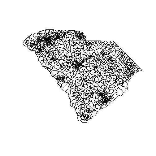

This is because plot “knows” what to do with shape data. In fact, we can explore this a little bit further:

class(precinct_shapes)

## [1] "SpatialPolygonsDataFrame"
## attr(,"package")
## [1] "sp"

This shows that we have an object of class sp, which is a spatial data object defined using the sp package. It is also a SpatialPolygonsDataFrame. Behind the scenes, plot is calling a method that is defined just for these kinds of objects, which tells it how to render these kinds of shape data. We could also (and have on this blog) done this using the ggplot2 package, but for this kind of exploration the quick plot is good. So don’t give completely up on R base graphics.

The election data has a bit of an odd structure.

DT::datatable(election_df %>% mutate(row=1:nrow(.)) %>% select(row,everything()) %>% slice(c(1:5,103:107)))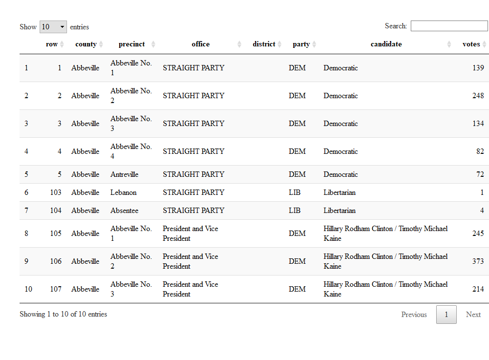

So the fancy stuff I did in kable above was basically to show the original row numbers and print them to the left of all the other variables. If I had not used the select(row,everything()), the row would have printed last. This is a nice example of how to do a quick custom column-sorting. But that’s not why we’re here. The election file shows how people voted in a rather raw fashion. Specifically, here I want to tally those people who voted for the different candidates for president. But it’s not that straightforward, because I have to count the straight-ticket voters as well as the split-party voters who specifically noted their president’s choice on the ballot.

The goal here is to get to the percentage of votes going to the big two parties. While it may be an interesting exercise to some to look at the third party votes, we’re not going to do that here.

total_pres_votes <- election_df %>% 
  filter(office %in% c("STRAIGHT PARTY","President and Vice President")) %>% 
  group_by(precinct) %>% 
  summarize(total_votes=sum(votes,nm.ra=TRUE))
DT::datatable(total_pres_votes)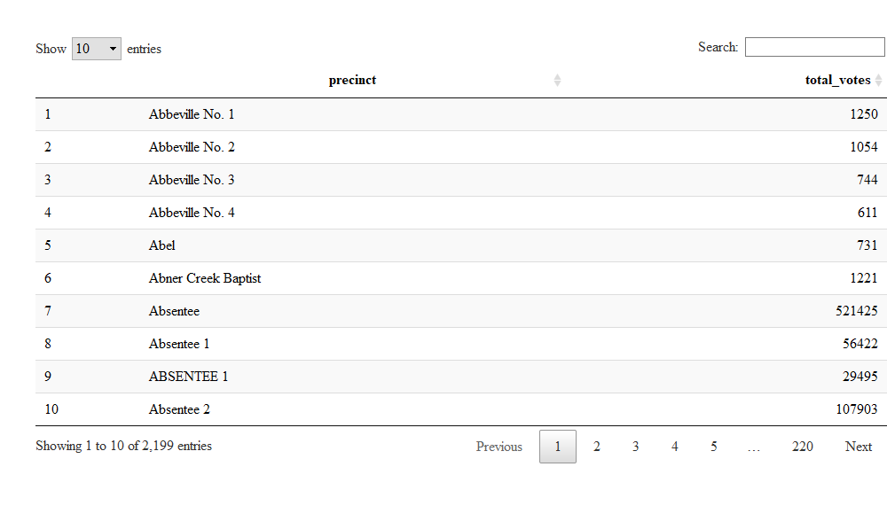

The first few results look ok, so we can get votes for the different parties and merge this back on to get the percentage.

total_party_votes <- election_df %>% 
  dplyr::filter((office %in% c("STRAIGHT PARTY","President and Vice President")) & (party %in% c("DEM","REP"))) %>% 
  group_by(precinct,party) %>% 
  summarize(total_party_votes=sum(votes,nm.ra=TRUE)) %>% 
  left_join(total_pres_votes) %>% 
  mutate(party_perc=total_party_votes/total_votes*100)

## Joining, by = "precinct"

DT::datatable(total_party_votes)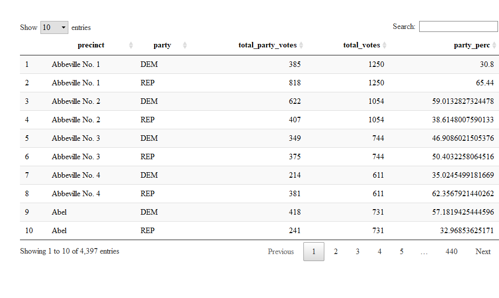

So one picky issue is worth mentioning here. This dataset counts absentee ballots as its own precinct (or their own precincts). Part of the joys of blogging is sweeping issues like this under the rug, but this can be the source of interesting analyses in their own right.

The final bit of data wrangling I do here is to widen the dataset, so I can merge it easily later on with the shapefile.

total_party_votes_wide <- total_party_votes %>% 
  select(-total_party_votes,-total_party_votes) %>% 
  group_by(precinct) %>% 
  spread(key=party,value=party_perc)
DT::datatable(total_party_votes_wide )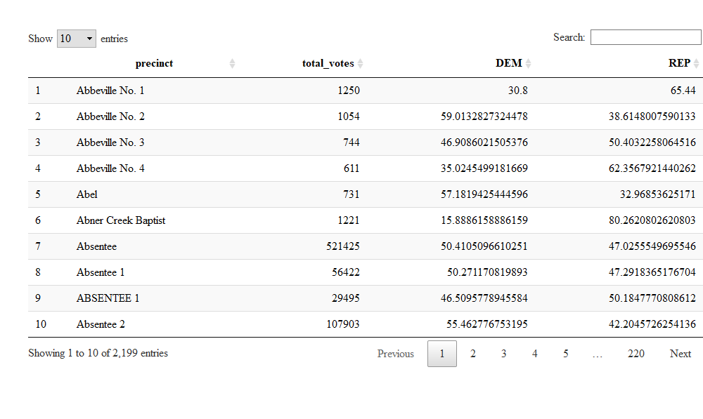

There were some casualties in this operation, namely the total party votes and total votes, but I don’t really need them for the simple thing I’m doing here.

The spread function I used above comes from the tidyr package, loaded by tidyverse. It, along with gather, enable navigating between “long” and “wide” datasets. You have to be careful using these functions, though, or you may get something strange. For instance, when I left in the party votes using spread above (in a previous iteration of this post), I ended up with an ugly wide and long dataset, but with NA every other row on each of the percent columns.

Merging data

In the last blog post, we were simply able to plot two maps on top of each other using the leaflet package. We are faced with a slightly different issue here. One data set is a geographic dataset, but the elections data only lists a precinct name. So it is up to us to do the merge.

precinct_elect <- merge(precinct_shapes,total_party_votes_wide,by.x="PNAME",by.y="precinct")

Honestly, I thought the above step would be the hardest part of the post. But like plot, the merge function in R understands what it’s operating on (i.e. uses a method that’s specific to spatial objects). Someone else did the hard work, and I just use the magic.

library(leaflet)
pal <- colorNumeric(palette = "viridis", 
                    domain = c(0,100))
 
precinct_elect %>% 
  leaflet(width="100%") %>% 
  addPolygons(popup = ~PNAME,
              stroke = FALSE,
                smoothFactor = 0,
                fillOpacity = 0.5,
                color = ~ pal(DEM)) %>% 
  addLegend("bottomright", 
              pal = pal, 
              values = ~ DEM,
              title = "Dem P/VP Vote %",
              labFormat = labelFormat(suffix = "%"),
              opacity = 1)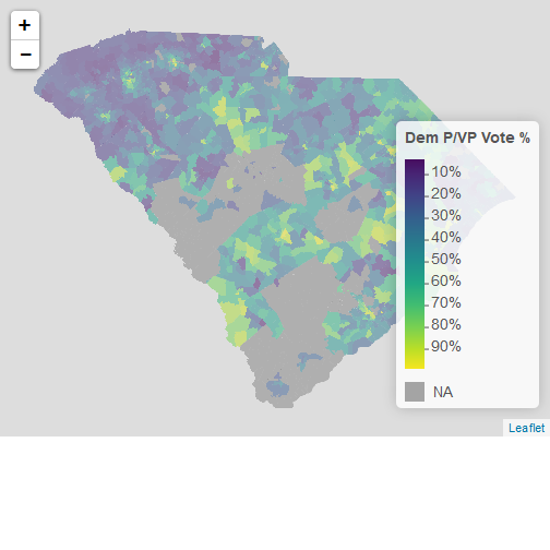

Now there are a few things to note:

• In this blog post, the map is static. If you actually run this code in RStudio, it will be an interactive map that lets you zoom and pan, and where clicking areas will give you the precinct name.
• I basically copied and pasted the leaflet code from the previous blog post, and changed variable names.
• It looks like the dataset has a few holes. This may be where sweeping the absentee ballot under the rug leaves out a lot.

Discussion

I used the data.world package and website to download and use Greenville election data. I then merged it with precinct shapefiles found from a different source (Github). The actual merge process wasn’t hard, and in fact the most difficult part of this process was deciding how I wanted to present the data. This election data is rather rich, but has a few necessary quirks in its structure.

Once you have characteristic data in the right format and shape files, it’s magically easy to merge them.

I copied and pasted most of the leaflet code from my last post to present the data, with tweaks for variable names.