In a previous post we plotted some points, retrieved from a public dataset in GeoJSON format, on top of a Google Map of the area surrounding Greenville, SC. In this post we plot some public data in GeoJSON format as well, but instead of particular points, we plot polygons. Polygons describe an area rather than a single point. As before, to set up we do the following:

library(rgdal)
if (!require(geojsonio)) {
    install.packages("geojsonio")
    library(geojsonio)
}
library(sp)
library(maps)
library(ggmap)
library(maptools)

Getting the data

The data we are going to analyze consists of the city parks in Greenville, SC. Though this data is located in an ArcGIS system, there is a GeoJSON version at OpenUpstate.

data_url <- "https://data.openupstate.org/maps/city-parks/parks.php"
data_file <- "parks.geojson"
# for some reason, I can't read from the url directly, though the tutorial
# says I can
download.file(data_url, data_file)
data_park <- geojson_read(data_file, what = "sp")

Analyzing the data

First, we plot the data as before:

plot(data_park)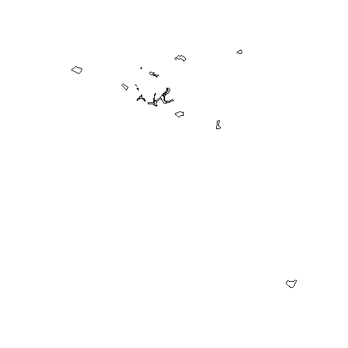

While this was easy to do, it doesn’t give very much context. However, it does give the boundaries of the different parks. As before, we use the ggmap and ggplot2 package to give us some context. First, we download from Google the right map.

mapImage <- ggmap(get_googlemap(c(lon = -82.394012, lat = 34.852619), scale = 1, 
    zoom = 11), extent = "normal")

I got the latitude and longitude by looking up on Google, and then hand-tuned the scale and zoom.

A note of warning: if you do this with a recent version of ggmap and ggplot2, you may need to download the GitHub versions. See this Stackoverflow thread for details.

Now, we prepare our spatial object for plotting. This is a more difficult process than before, and requires the use of the fortify command from ggplot2 package to make sure everything makes it to the right format:

data_park_df <- fortify(data_park)

Now we can make the plot:

print(mapImage + geom_polygon(aes(long, lat, group = group), data = data_park_df, 
    colour = "green"))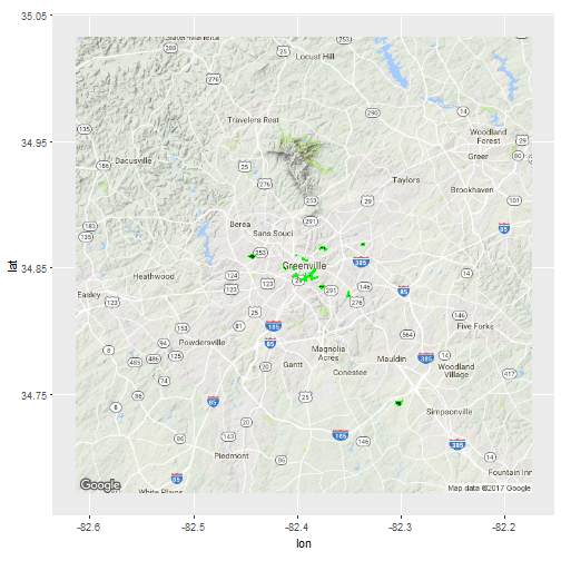

Note the use of the group= option in the geom_polygon function above. This tells geom_polygon that there are many polygons rather than just one. Without that option, you get a big mess:

print(mapImage + geom_polygon(aes(long, lat), data = data_park_df, colour = "green"))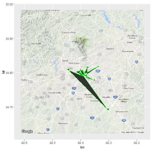

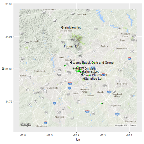
Mashup of parking convenient to Swamp Rabbit Trail and city parks

Now, say you want to combine the city parks data with the parking places convenient to Swamp Rabbit Trail that was the subject of the last post. That is very easy using the ggplot2 package. We get the data and manipulate it as last time:

Next, we use the layering feature of ggplot2 to draw the map:

Conclusions

We continue to explore public geographical data by examining data representing areas in addition to points. In addition, we layer data from two sources.