GeoJSON is a standard text-based data format for encoding geographical information, which relies on the JSON (Javascript object notation) standard. There are a number of public datasets for Greenville, SC that use this format, and, the R programming language makes working with these data easy. Install the rgeojson library, which is part of the ROpenSci family of packages.

In this post we plot some public data in GeoJSON format on top of a retrieved Google Map. To set up we do the following:

library(rgdal)
if (!require(geojsonio)) {
    install.packages("geojsonio")
    library(geojsonio)
}
library(sp)
library(maps)
library(ggmap)
library(maptools)

I wrapped geojsonio in a require because it may not be installed on your system. Geojsonio takes most of the work out of dealing with GeoJSON data, thus allowing you to concentrate on your analysis rather than data manipulation to a great extent. There is still some data manipulation to be done, as seen below, but it’s fairly lightweight.

Getting the data

The data we are going to analyze consists of the convenient parking locations for access to the Swamp Rabbit Trail running between Greenville, SC and Traveler’s Rest, SC. Though this data is located in an ArcGIS system, there is a GeoJSON version at OpenUpstate.

data_url <- "https://data.openupstate.org/maps/swamp-rabbit-trail/parking/geojson.php"
data_file <- "srt_parking.geojson"
# for some reason, I can't read from the url directly, though the tutorial
# says I can
download.file(data_url, data_file)
data_json <- geojson_read(data_file, what = "sp")

Theoretically, you can use geojson_read to get the data from the URL directly; however this seemed to fail for me. I’m not sure why doing the two-step process with download.file and then geojson_read works, but it is probably a good idea to download your data first in most cases. The what="sp" option in geojson_read is used to return the data in a spatial object. Now that the data is in a spatial object, we can analyze however we wish and forget about the original data format.

Analyzing the data

The first thing you can do is plot the data, and the plot command makes that easy. If you don’t know what is going on behind the scenes, the plot command detects that it is dealing with a spatial object and calls the plot method from the sp package. But we just issue a simple command:

plot(data_json)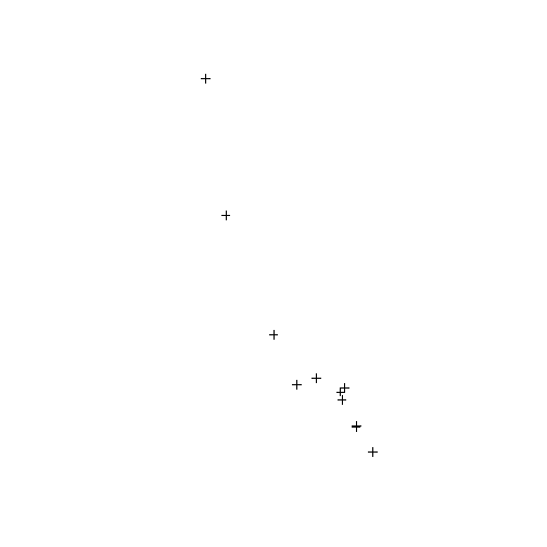

Unfortunately, this plot is not very helpful because it simply plots the points without any context. So we use the ggmap and ggplot2 package to give us some context. First, we download from Google the right map.

mapImage <- ggmap(get_googlemap(c(lon = -82.394012, lat = 34.852619), scale = 1, 
    zoom = 11), extent = "normal")

I got the latitude and longitude by looking up on Google, and then hand-tuned the scale and zoom.

A note of warning: if you do this with a recent version of ggmap and ggplot2, you may need to download the GitHub versions. See this Stackoverflow thread for details.

Now, we prepare our spatial object for plotting:

data_df <- as.data.frame(data_json)
names(data_df)[4:5] <- c("lon", "lat")

There’s really no output from this. I suppose the renaming step isn’t necessary, but I believe in descriptive labels.

Now we can make the plot:

print(mapImage + geom_point(aes(lon, lat), data = data_df))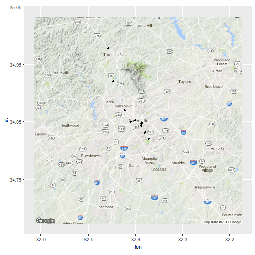

It may be helpful to add labels based on the name of the location, given in the ‘title’ field:

mapImage + geom_point(aes(lon, lat), data = data_df) + geom_text(aes(lon, lat, 
    label = title, hjust = 0, vjust = 0.5), data = data_df, check_overlap = TRUE)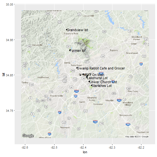

Here, I use geom_text to make the labels, and tweaked the options by hand using the help page.

Conclusions

GeoJSON data is becoming more popular, especially in public data. The geojsonio package makes working with such data trivial. Once the data is in a spatial data format, R’s wide variety of spatial data tools are available.