
How to make maps with Census data in R
US Census Data
The US Census collects a number of demographic measures and publishes aggregate data through its website. There are several ways to use Census data in R, from the Census API to the USCensus2010 package. If you are interested in geopolitical data in the US, I recommend exploring both these options - the Census API requires a key for each person who uses it, and the package requires downloading a very large dataset. The setups for both require some effort, but once that effort is done you don’t have to do it again.
The acs package in R allows you to access the Census API easily. I highly recommend checking it out, and that’s the method we will use here. Note that I’ve already defined the variable api_key - if you are trying to run this code you will need to first run something like api_key <- <enter your Census API key> before running the rest of this code.
library(acs)
api.key.install(key=api_key) # now you are ready to run the rest of the acs code
For purposes here, we will use the toy example of plotting median household income by county for every county in South Carolina. First, we obtain the Census data. The first command gives us the table and variable names of what we want. I then use that table number in the acs.fetch command to get the variable I want.
acs.lookup(endyear=2015, span=5,dataset="acs", keyword= c("median","income","family","total"), case.sensitive=F)## Warning in acs.lookup(endyear = 2015, span = 5, dataset = "acs", keyword = c("median", : XML variable lookup tables for this request
## seem to be missing from ' https://api.census.gov/data/2015/acs5/variables.xml ';
## temporarily downloading and using archived copies instead;
## since this is *much* slower, recommend running
## acs.tables.install()## An object of class "acs.lookup"
## endyear= 2015 ; span= 5
##
## results:
## variable.code table.number
## 1 B10010_001 B10010
## 2 B19126_001 B19126
## 3 B19126_002 B19126
## 4 B19126_005 B19126
## 5 B19126_006 B19126
## 6 B19126_009 B19126
## 7 B19215_001 B19215
## 8 B19215_002 B19215
## 9 B19215_003 B19215
## 10 B19215_006 B19215
## 11 B19215_009 B19215
## 12 B19215_010 B19215
## 13 B19215_013 B19215
## table.name
## 1 Median Family Income for Families with GrndPrnt Householders Living With Own GrndChldrn < 18 Yrs
## 2 B19126. Median Family Income in the Past 12 Months (in 2015 Inflation-Adjusted Dollars) by Family Type by Presence of Own Children Under 18 Years
## 3 B19126. Median Family Income in the Past 12 Months (in 2015 Inflation-Adjusted Dollars) by Family Type by Presence of Own Children Under 18 Years
## 4 B19126. Median Family Income in the Past 12 Months (in 2015 Inflation-Adjusted Dollars) by Family Type by Presence of Own Children Under 18 Years
## 5 B19126. Median Family Income in the Past 12 Months (in 2015 Inflation-Adjusted Dollars) by Family Type by Presence of Own Children Under 18 Years
## 6 B19126. Median Family Income in the Past 12 Months (in 2015 Inflation-Adjusted Dollars) by Family Type by Presence of Own Children Under 18 Years
## 7 B19215. Median Nonfamily Household Income in the Past 12 Months (in 2015 Inflation-Adjusted Dollars) by Sex of Householder by Living Alone by Age of Householder
## 8 B19215. Median Nonfamily Household Income in the Past 12 Months (in 2015 Inflation-Adjusted Dollars) by Sex of Householder by Living Alone by Age of Householder
## 9 B19215. Median Nonfamily Household Income in the Past 12 Months (in 2015 Inflation-Adjusted Dollars) by Sex of Householder by Living Alone by Age of Householder
## 10 B19215. Median Nonfamily Household Income in the Past 12 Months (in 2015 Inflation-Adjusted Dollars) by Sex of Householder by Living Alone by Age of Householder
## 11 B19215. Median Nonfamily Household Income in the Past 12 Months (in 2015 Inflation-Adjusted Dollars) by Sex of Householder by Living Alone by Age of Householder
## 12 B19215. Median Nonfamily Household Income in the Past 12 Months (in 2015 Inflation-Adjusted Dollars) by Sex of Householder by Living Alone by Age of Householder
## 13 B19215. Median Nonfamily Household Income in the Past 12 Months (in 2015 Inflation-Adjusted Dollars) by Sex of Householder by Living Alone by Age of Householder
## variable.name
## 1 Median family income in the past 12 months-- Total:
## 2 Median family income in the past 12 months (in 2015 Inflation-adjusted dollars) -- Total:
## 3 Median family income in the past 12 months (in 2015 Inflation-adjusted dollars) -- Married-couple family -- Total
## 4 Median family income in the past 12 months (in 2015 Inflation-adjusted dollars) -- Other family -- Total
## 5 Median family income in the past 12 months (in 2015 Inflation-adjusted dollars) -- Other family -- Male householder, no wife present -- Total
## 6 Median family income in the past 12 months (in 2015 Inflation-adjusted dollars) -- Other family -- Female householder, no husband present -- Total
## 7 Median nonfamily household income in the past 12 months (in 2015 Inflation-adjusted dollars) -- Total (dollars):
## 8 Median nonfamily household income in the past 12 months (in 2015 Inflation-adjusted dollars) -- Male householder -- Total (dollars)
## 9 Median nonfamily household income in the past 12 months (in 2015 Inflation-adjusted dollars) -- Male householder -- Living alone -- Total (dollars)
## 10 Median nonfamily household income in the past 12 months (in 2015 Inflation-adjusted dollars) -- Male householder -- Not living alone -- Total (dollars)
## 11 Median nonfamily household income in the past 12 months (in 2015 Inflation-adjusted dollars) -- Female householder -- Total (dollars)
## 12 Median nonfamily household income in the past 12 months (in 2015 Inflation-adjusted dollars) -- Female householder -- Living alone -- Total (dollars)
## 13 Median nonfamily household income in the past 12 months (in 2015 Inflation-adjusted dollars) -- Female householder -- Not living alone -- Total (dollars)my_cnty <- geo.make(state = 45,county = "*")
home_median_price<-acs.fetch(geography=my_cnty, table.number="B19126",endyear=2015) # home median prices## Warning in (function (endyear, span = 5, dataset = "acs", keyword, table.name, : XML variable lookup tables for this request
## seem to be missing from ' https://api.census.gov/data/2015/acs5/variables.xml ';
## temporarily downloading and using archived copies instead;
## since this is *much* slower, recommend running
## acs.tables.install()## Error in if (url.test["statusMessage"] != "OK") {: missing value where TRUE/FALSE neededknitr::kable(head(home_median_price@estimate))| B19126_001 | B19126_002 | B19126_003 | B19126_004 | B19126_005 | B19126_006 | B19126_007 | B19126_008 | B19126_009 | B19126_010 | B19126_011 | |
|---|---|---|---|---|---|---|---|---|---|---|---|
| Abbeville County, South Carolina | 44918 | 55141 | 65664 | 50698 | 24835 | 43187 | 50347 | 24886 | 22945 | 18101 | 29958 |
| Aiken County, South Carolina | 57396 | 70829 | 72930 | 70446 | 29302 | 36571 | 35469 | 37906 | 27355 | 22760 | 34427 |
| Allendale County, South Carolina | NA | NA | NA | NA | NA | NA | NA | NA | NA | NA | NA |
| Anderson County, South Carolina | 53169 | 65881 | 75444 | 60166 | 26608 | 36694 | 37254 | 36297 | 24384 | 17835 | 29280 |
| Bamberg County, South Carolina | NA | NA | NA | NA | NA | NA | NA | NA | NA | NA | NA |
| Barnwell County, South Carolina | 44224 | 59467 | 70542 | 54030 | 19864 | 25143 | 18633 | 45714 | 18317 | 13827 | 21315 |
Plotting the map data
If you have the maps and ggplot2 packages, you already have the data you need to plot. We use the map_data function from ggplot2 to pull in county shape data for South Carolina. (A previous attempt at this blogpost had used the ggmap package, but there is an incompatibility between that and the latest ggplot2 package at the time of this writing.)
library(ggplot2)## Want to understand how all the pieces fit together? Buy the
## ggplot2 book: http://ggplot2.org/book/sc_map <- map_data("county",region="south.carolina")
ggplot() + geom_polygon(aes(x=long,y=lat,group=group),data=sc_map,colour="white",fill="black") + theme_minimal()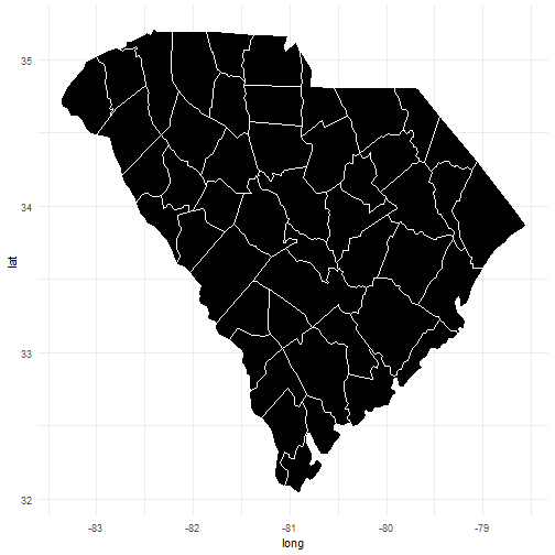
Merging the demographic and map data
Now we have the demographic data and the map, but merging the two will take a little effort. The reason is that the map data gives a lower case representation of the county and calls it a “subregion”, while the Census data returns the county as “xxxx County, South Carolina”. I use the dplyr and stringr packages (for str_replace) to make short work of this merge.
library(dplyr)
library(stringr)

merged <- as.data.frame(home_median_price@estimate) %>%
  mutate(county_full = rownames(.),
         county = str_replace(county_full,"(.+) County.*","\\1") %>% tolower) %>%
  select(county,B19126_001) %>%
  rename(med_income=B19126_001) %>%
  right_join(sc_map,by=c("county"="subregion"))

knitr::kable(head(merged,10))| county | med_income | long | lat | group | order | region |
|---|---|---|---|---|---|---|
| abbeville | 44918 | -82.24809 | 34.41758 | 1 | 1 | south carolina |
| abbeville | 44918 | -82.31685 | 34.35455 | 1 | 2 | south carolina |
| abbeville | 44918 | -82.31111 | 34.33163 | 1 | 3 | south carolina |
| abbeville | 44918 | -82.31111 | 34.29152 | 1 | 4 | south carolina |
| abbeville | 44918 | -82.28247 | 34.26860 | 1 | 5 | south carolina |
| abbeville | 44918 | -82.25955 | 34.25142 | 1 | 6 | south carolina |
| abbeville | 44918 | -82.24809 | 34.21131 | 1 | 7 | south carolina |
| abbeville | 44918 | -82.23663 | 34.18266 | 1 | 8 | south carolina |
| abbeville | 44918 | -82.24236 | 34.15401 | 1 | 9 | south carolina |
| abbeville | 44918 | -82.27674 | 34.10818 | 1 | 10 | south carolina |
It’s now a simple matter to plot this merged dataset. In fact, we only have to tweak a few things from the first time we plotted the map data.
ggplot() + geom_polygon(aes(x=long,y=lat,group=group,fill=med_income),data=merged) + theme_minimal()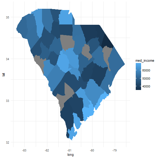
Discussion
It’s pretty easy to plot U.S. Census data on a map. The real power of Census data comes not just from plotting it, but combining with other geographically-based data (such as crime). The acs package in R makes it easy to obtain Census data, which can then be merged with other data using packages such as dplyr and stringr and then plotted with ggplot2. Hopefully the authors of the ggmap and ggplot2 packages can work out their incompatibilities so that the above maps can be created using the Google API map or open street maps.
It should be noted that while I obtained county-level information, aggregate data can be obtained at Census block and tract levels as well, if you are looking to do some sort of localized analysis.