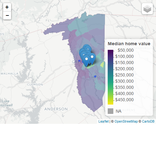
So the goal here is to focus back on Greenville County and have even more granularity. I look at median house prices near Greenville and then overlay the park data downloaded earlier. This time, for the Census data, I use the tidycensus package that came out recently. Furthermore, instead of using ggplot2 to create a static map, I use the leaflet package to create an interactive map, and, furthermore integrate data from disparate sources in a convenient way.

Download the local park data

The local parks file can be found here courtesy of a small group of dedicated volunteers and an API that makes publishing geojson files easy at the Open Upstate site. We will download a polygon file for the park boundaries as well as a point geojson file for the address of each park.

data_url <- "https://data.openupstate.org/maps/city-parks/parks.php"
data_file <- "parks.geojson"
# for some reason, I can't read from the url directly, though the tutorial
# says I can
download.file(data_url, data_file)
data_park <- geojson_read(data_file, what = "sp")
 
data_url <- "https://data.openupstate.org/maps/city-parks/geojson.php"
data_file <- "parks_point.geojson"
# for some reason, I can't read from the url directly, though the tutorial
# says I can
download.file(data_url, data_file)
data_park_addr <- geojson_read(data_file, what = "sp")

Download the median home value data

This code from tidycensus downloads demographic data and geometric data in a list column. A list column is a data frame, but one of the variables really contains a spatial data frame for each observation, which gives the polygon data for the census tracts. Having the demographic and geometric data in this format eases bookkeeping, and, thankfully, leaflet understands this format.

gvl_value <- get_acs(geography = "tract", 
                    variables = "B25077_001", 
                    state = "SC",
                    county = "Greenville County",
                    geometry = TRUE)

Plot the census and local data together

Now we bring everything together. The leaflet package was written to make extensive use of the pipe operator that dplyr introduced a few years ago. We can set a default data frame for a leaflet map, but when we add markers and polygons, we can set it from other data sources. The following code is one way to do this, where we use the tidycensus-generated dataset as the foundation of the leaflet. We add polygons and markers for the data park using the data= option of addPolygons and addMarkers. Note the use of the group= option to create layers, which can be clicked on and off interactively. The label= option (or popup= option for addPolygons) are used to generate popup windows that give additional information.

pal <- colorNumeric(palette = "viridis", 
                    domain = gvl_value$estimate)
 
gvl_value %>%
    st_transform(crs = "+init=epsg:4326") %>%
    leaflet(width = "100%") %>%
    addProviderTiles(provider = "CartoDB.Positron") %>%
    addPolygons(popup = ~ str_extract(NAME, "^([^,]*)"),
                stroke = FALSE,
                smoothFactor = 0,
                fillOpacity = 0.5,
                color = ~ pal(estimate),
                group="Median home value") %>%
    addLegend("bottomright", 
              pal = pal, 
              values = ~ estimate,
              title = "Median home value",
              labFormat = labelFormat(prefix = "$"),
              opacity = 1) %>% 
  addPolygons(data=data_park,fillOpacity=0.8,group="Parks") %>% 
  addMarkers(data=data_park_addr,group="Parks",label=~title) %>% 
  addLayersControl(overlayGroups = c("Parks","Median home value"))

Unfortunately due to the limitations of Github pages this had to be turned into a static image to be rendered. Perhaps it’s time to make the jump to blogdown and hugo like all the other cool kids?

Discussion

I’m just starting to learn about the leaflet package, but in just a couple of hours (and standing on the shoulders of giants) I was able to put together an interactive map combining Census data (median home value by census tract) and locally-generated data (park locations). Such combinations can be effectively used to examine local situations in the context of rich data already collected at a federal level (assuming the instability at the U.S. Census Bureau is temporary).