
Greenville on Twitter
In this blogpost, we use R to use Twitter data to analyze topics of interest to Greenville, SC. We will describe obtaining, manipulating, and summarizing the data.
Twitter is a “microblogging” service where users can, usually publicly, share links, pictures, or short comments (up to 140 characters) onto a timeline. The public timeline consists of all public tweets, but people can build their own private timelines to narrow content to just what they want to see. (They do this by “following” users.) Over the years, many companies, news organizations, and users have considered the social media site essential for sharing news and other information. (Or cat memes.) Twitter has some organizational tools such as replies/conversation threads, mentions (i.e. naming other users using the @ notation), and hashtags (naming a topic using # notation). Twitter has encouraged the use of these organizational tools by automatically making mentions and hashtags clickable links.
These organizational tools can make for some interesting analysis. For instance, a game show may encourage viewers to vote on a winner using hashtags. On their end, they create a filter for a particular hashtag (e.g. #votemyplayer) and count votes. This also makes Twitter data ripe for text mining (which they use to identify trending topics).
Obtaining the Twitter data
Twitter makes it possible for software to obtain Twitter comments without having to resort to “web-scraping” techniques (i.e. downloading the data as a web page and then parsing the HTML). Instead, you can go through an Application Programming Interface (API) to obtain the comments directly. If you’re interested, Twitter has a whole subdomain related to accessing their data, including documentation. There are a lot of technical details, but for the casual user probably the only ones of interest are API key and rate limits. This post won’t fuss with rate limits, but more serious work may require some further understanding of these issues. However, you will need to create an API key. Follow these instructions, which are tailored for R users. It essentially consists of creating a token at Twitter’s app web site and running an R function with the token. I set variables consumer_secret, consumer_key, access_token, and access_secret in an R block just copying and pasting from the Twitter apps site, not echoed in this blog post for obvious reasons.
Fortunately, the twitteR package makes obtaining data from Twitter easy. It’s on CRAN, so grab it using install.packages (it will also install dependencies such as the bit64 and httr packages if you don’t have them already) before moving on.
We authenticate our R program to Twitter and then start with searching the public timeline for “Greenville”. Note due to the changing nature of Twitter, your results will probably be different:
origop <- options("httr_oauth_cache")
options(httr_oauth_cache = TRUE)
library(twitteR)
setup_twitter_oauth(consumer_key, consumer_secret, access_token, access_secret)
[1] "Using direct authentication"options(httr_oauth_cache = origop)
gvl_twitter <- searchTwitter("Greenville")
gvl_twitter_df <- twListToDF(gvl_twitter)
head(gvl_twitter_df) text
1 RT @JessLivMo: PROTEST: Greenville TODAY at 4pm! https://t.co/PtDqfV1iQi
2 Y'all, #texaspawprints is at the Pet Supplies on lower Greenville today. Their kitties areÂ… https://t.co/AVwAEvm9w5
3 RT @nssottile: What is Governor @henrymcmaster doing to get Greenville resident and Clemson Ph.D. #NazaninZinouri back home? #sctweets #MusÂ…
4 Can you recommend anyone for this #job in #Greenville, SC? https://t.co/bGoRU5wFqQ #Labor #Hiring #CareerArc
favorited favoriteCount replyToSN created truncated
1 FALSE 0 <NA> 2017-01-29 20:07:33 FALSE
2 FALSE 0 <NA> 2017-01-29 20:06:10 FALSE
3 FALSE 0 <NA> 2017-01-29 20:05:53 FALSE
4 FALSE 0 <NA> 2017-01-29 20:04:47 FALSE
replyToSID id replyToUID
1 <NA> 825797550087217152 <NA>
2 <NA> 825797204724088836 <NA>
3 <NA> 825797131420053505 <NA>
4 <NA> 825796855728451584 <NA>
statusSource
1 <a href="http://www.samruston.co.uk" rel="nofollow">Flamingo for Android</a>
2 <a href="http://linkis.com" rel="nofollow">Put your button on any page! </a>
3 <a href="http://twitter.com/download/iphone" rel="nofollow">Twitter for iPhone</a>
4 <a href="http://www.tweetmyjobs.com" rel="nofollow">TweetMyJOBS</a>
screenName retweetCount isRetweet retweeted longitude
1 RatherBeGulfing 15 TRUE FALSE <NA>
2 KickButtVegan 0 FALSE FALSE -96.77009998
3 ClaireOfTarth 47 TRUE FALSE <NA>
4 tmj_grn_labor 0 FALSE FALSE -82.4536115
latitude
1 <NA>
2 32.81234958
3 <NA>
4 34.8268335
[ reached getOption("max.print") -- omitted 2 rows ]searchTwitter returns data as a list, which may or may not be desirable. As a default, it returns the last 25 items matching the query you pass (this can be changed by using the n= option to the function). I used twListToDF (part of the twitteR package) to convert to a data frame. The data frame contains a lot of useful information, such as the tweet, information about whether it’s a reply and the tweet to which it’s a reply, screen name, and date stamp. Thus, Twitter provides a rich data source to provide information on topics, interactions, and reactions.
Analyzing the data
Retweets
The first thing to notice is that many of these tweets may be “retweets”, where a user posts the exact same tweet as a previous user to create a larger audience for the tweet. This data point may be interesting in its own right, but for now, because we are just analyzing the text, we will filter out retweets:
library(dplyr)
gvl_twitter_unique <- gvl_twitter_df %>% filter(!isRetweet)

print(gvl_twitter_unique %>% select(text))
text
1 Y'all, #texaspawprints is at the Pet Supplies on lower Greenville today. Their kitties areÂ… https://t.co/AVwAEvm9w5
2 Can you recommend anyone for this #job in #Greenville, SC? https://t.co/bGoRU5wFqQ #Labor #Hiring #CareerArc
3 @Meghan_Trainor i miss u <ed><U+00A0><U+00BD><ed><U+00B8><U+00AD><ed><U+00A0><U+00BD><ed><U+00B8><U+00AD>\nCome back to Greenville soon <U+2764>
4 1/29/73 Greenville, SC. Bobby & Terry Kay vs Freddy Sweetan/Mike DuBois, Johnny Weaver/Penny Banner vs The Alaskan/Â… https://t.co/hFH3iCeWLl
5 Interested in a #job in #Greenville, SC? This could be a great fit: https://t.co/yuufbTYC57 #IT #Hiring #CareerArc
6 Join the Robert Half Technology team! See our latest #job opening here: https://t.co/xCNLSvTkDQ #RHTechJobs #IT #Greenville, SC #Hiring
7 Want to work at Hubbell Incorporated? We're #hiring in #Greenville, SC! Click for details: https://t.co/dfTOjYDWG9 #Job #ProductMgmt #Jobs
8 I need a church in Greenville ASAP! If you have suggestions let me know
9 Wow! @Lyft pledges $1 million to @ACLU https://t.co/YTkkGeE5l6 #Lyft is finally in Greenville. App downloaded. #DeleteUber
10 Greenville, NC: 3:00 PM Temp: 53.5ºF Dew: 25.8ºF Pressure: 1008.2mb Rain: 0.00" #encwx #ncwx https://t.co/sZnc3rvVsm
11 Interested in a #job in #Dearborn, MI? This could be a great fit: https://t.co/GxLvH7wJ9J #Retail #Hiring #CareerArc
12 Want to work in #Greenville, NC? View our latest opening: https://t.co/aU11faXsxp #Job #Healthcare #Jobs #Hiring #CareerArc
13 Driving to Greenville, sharing real-time road info with wazers in my area. ETA 3:23 PM using @waze - Drive Social.
14 #Pursue #Bright #Career With The #Universities In #South #Australia\n\nhttps://t.co/ZD6nPXglKr\n#CheapFlights #Greenville
15 https://t.co/DVdFrLQwaF\nMy latest Greenville News column.
16 @igorvolsky Greenville-Spartanburg, South Carolina (GSP), today at 4:00.
17 Join the WHBM team! See our latest #job opening here: https://t.co/jd5D8zjYXW #Retail #Greenville, SC #Hiring #CareerArc
18 (Greenville, SC) I need to figure out what happened to my driver's license, or I'm going to los... https://t.co/CS4qMYpUkB
19 See our latest #Greenville, SC #job and click to apply: Mortgage Consultant (SAFE) - https://t.co/f9H5PO30Fe #Veterans #Hiring #CareerArcThe thing to notice here is that there are several different Greenvilles, so this makes analysis of the local area pretty hard. Many of the tweets can be about Greenville, NC or SC. In this particular dataset, there was even a Greenville Road in California (where there was a car fire). Rather than play a filtering game, it may be better to apply some knowledge specific to the area. For instance, local tweets will often be tagged with #yeahThatgreenville. So we will search again for the #yeahthatgreenville hashtag (and add a few more tweets as well). This time, we’ll keep retweets:
origop <- options("httr_oauth_cache")
options(httr_oauth_cache = TRUE)
setup_twitter_oauth(consumer_key, consumer_secret, access_token, access_secret)  # needed to knit the Rmd file, may not be necessary for you to reauthenticate in 1 session
[1] "Using direct authentication"options(httr_oauth_cache = origop)
gvl_twitter_unique <- searchTwitter("#yeahthatgreenville", n = 200) %>% twListToDF()
gvl_twitter_nolink <- gvl_twitter_unique %>% mutate(text = gsub("https?://[\\w\\./]+",
"", text, perl = TRUE))Here I do two separate queries and add them together using the bind_rows function from dplyr.
Who is tweeting
The first thing we can do is get a list of users who tweet under this hastag as well as their number of tweets:
library(ggplot2)

gvl_twitter_nolink %>% ggplot(aes(x = reorder(screenName, screenName, function(x) -length(x)))) +
    geom_bar() + theme(axis.text.x = element_text(angle = 60, hjust = 1)) +
    xlab("")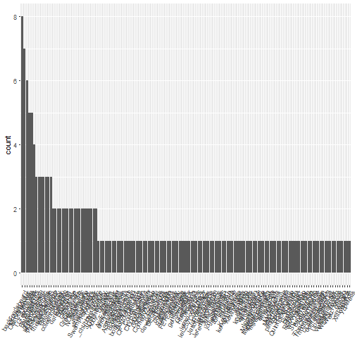
So I snuck a trick into the above graph. In bar charts presenting counts, I usually prefer the order in descending bar length. That way I can identify the most and least common screen names quickly. I accomplish this by using x=reorder(screenName,screenName,function (x) -length(x))) in the aes() function above. Now we can see that @GiovanniDodd was the most prolific tweeter in the last 200 tweets I accessed. Some of the prolific tweeters appear to be businesses, such as @CourtyardGreenville or perhaps tourism accounts such as @Greenville_SC.
What users are saying
To analyze what users are saying about “#yeahthatgreenville”, we use the tidytext package. There are a number of packages that can be used to analyze text, and tm used to be a favorite, but tidytext fits within the context of tidy data. We prefer the tidy data framework because it works with data in a specific format and has a number of powerful tools that have a specific focus but interoperate well, much like the UNIX ideal. Here, tidytext will allow us to use dplyr and similar tools using the pipe operator. The code will be easier to read and follow.
library(tidytext)

tweet_words <- gvl_twitter_nolink %>% select(id, text) %>% unnest_tokens(word,
    text)

head(tweet_words)
id word
1 825791100107505664 tonight
1.1 825791100107505664 at
1.2 825791100107505664 coffee
1.3 825791100107505664 underground
1.4 825791100107505664 1
1.5 825791100107505664 eI used the select function from dplyr to keep only the id and text fields. The unnest_tokens() functions creates a long dataset with a single word replacing the text. All the other fields remain unchanged. We can now easily create a bar chart of the words used the most:
tweet_words %>% ggplot(aes(x = reorder(word, word, function(x) -length(x)))) +
    geom_bar() + theme(axis.text.x = element_text(angle = 60, hjust = 1)) +
    xlab("")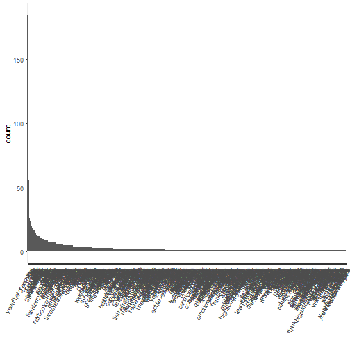
This plot is very busy, so we plot, say, the top 20 words:
tweet_words %>% count(word, sort = TRUE) %>% slice(1:20) %>% ggplot(aes(x = reorder(word,
    n, function(n) -n), y = n)) + geom_bar(stat = "identity") + theme(axis.text.x = element_text(angle = 60,
    hjust = 1)) + xlab("")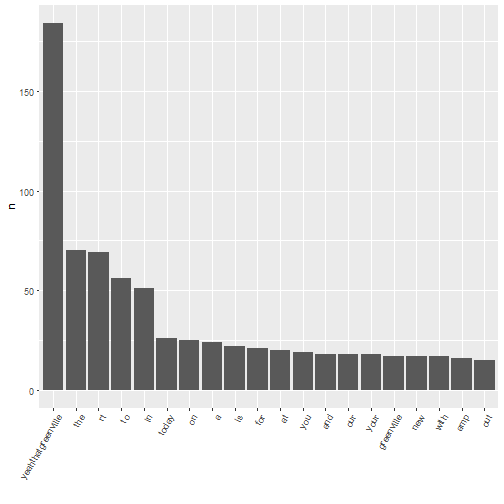
Unfortunately, this is terribly unexciting. Of course “a”, “to”, “for”, and similar words are going to be at the top. In text mining, we create a list of “stop words”, including these, which are so common they are usually not worth including in an analysis. The tidytext package includes a stop_words data frame to assist us:
head(stop_words)# A tibble: 6 × 2
word lexicon
<chr> <chr>
1 a SMART
2 a's SMART
3 able SMART
4 about SMART
5 above SMART
6 according SMARTWe’ll change stop_words slightly to be useful to us. This involves adding a column to help us filter out in the next step and adding some common, uninteresting words “https”, “t.co”, “yeahthatgreenville”, and “amp”. We filter these out for various reasons, e.g. “https” and “t.co” are used in URLs, “amp” is left over from tokening some HTML code, and we searched on “yeahthatgreenville”. Augmenting stop words is a bit of an iterative process, which I’m not showing here, but I went back and forth a few times to get this list.
my_stop_words <- stop_words %>% select(-lexicon) %>% bind_rows(data.frame(word = c("https",
    "t.co", "yeahthatgreenville", "amp", "gvl")))
Now, we can determine which of the words above are stop words and thus not worth analyzing:
tweet_words_interesting <- tweet_words %>% anti_join(my_stop_words)

head(tweet_words_interesting)
id word
1 825791100107505664 tonight
2 825474845710376962 tonight
3 825443843445293057 tonight
4 825791100107505664 coffee
5 825791100107505664 coffee
6 825693272119054336 coffeeThe anti_join function is probably not familiar to most data scientists or statisticians. It is the opposite of a merge in a sense. Basically, the command above merges the tweet_words and my_stop_words data frames, and then removes the rows that came from the my_stop_words dataset, leaving only the rows in tweet_words (the id and word) that does not match with something from my_stop_words. This is desirable because our my_stop_words dataset contains words we do not want to analyze.
Now we can analyze the more interesting words:
tweet_words_interesting %>% count(word, sort = TRUE) %>% slice(1:20) %>% ggplot(aes(x = reorder(word,
    n, function(n) -n), y = n)) + geom_bar(stat = "identity") + theme(axis.text.x = element_text(angle = 60,
    hjust = 1)) + xlab("")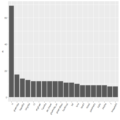
Sentiment analysis
Sentiment analysis is, in short, the quantitative study of the emotional content of text. The most sophisticated analysis, of course, is very difficult, but we can make a start using a simple procedure. Many of the ideas here can be found in a vignette for the package written by Julia Silge and David Robinson.
As a start, we use the Bing lexicon, which maps a word to positive/negative according to whether its sentiment content is positive or negative.
bing_lex <- get_sentiments("bing")

head(bing_lex)
# A tibble: 6 × 2
word sentiment
<chr> <chr>
1 2-faced negative
2 2-faces negative
3 a+ positive
4 abnormal negative
5 abolish negative
6 abominable negativeSentiment analysis then is an exercise in an inner-join:
gvl_sentiment <- tweet_words_interesting %>% left_join(bing_lex)

head(gvl_sentiment)
id word sentiment
1 825791100107505664 tonight <NA>
2 825474845710376962 tonight <NA>
3 825443843445293057 tonight <NA>
4 825791100107505664 coffee <NA>
5 825791100107505664 coffee <NA>
6 825693272119054336 coffee <NA>Once you get to this point, sentiment analysis can start fairly easily:
gvl_sentiment %>% filter(!is.na(sentiment)) %>% group_by(sentiment) %>% summarise(n = n())# A tibble: 2 × 2
sentiment n
<chr> <int>
1 negative 25
2 positive 96There are many more positive words than negative words, so the mood tilts positive in our crude analysis. We can also group by tweet, and see whether there more more positive or negative tweets:
gvl_sent_anly2 <- gvl_sentiment %>% group_by(sentiment, id) %>% summarise(n = n()) %>%
    ungroup() %>% group_by(sentiment) %>% summarise(n = mean(n, na.rm = TRUE))

gvl_sent_anly2
# A tibble: 3 × 2
sentiment n
<chr> <dbl>
1 negative 1.041667
2 positive 1.333333
3 <NA> 6.361809On average, there are 1.3333333 positive words per tweet and 1.0416667 negative words per tweet, if you accept the assumptions of the above analysis.
There is, of course, a lot more that can be done, but this will get you started. For some more sophisticated ideas you can check Julia Silge’s analysis of Reddit data, for instance. Another kind of analysis looking at sentiment and emotional content can be found here (with the caveat that it uses the predecessor to dplyr and thus runs somewhat less efficiently). Finally, it would probably be useful to supplement the above sentiment data frames with situation-specific sentiment analysis, such as making goallllllll in the above a positive word.
Conclusions
The R packages twitteR and tidytext make analyzing content from Twitter easy. This is helpful if you want to analyze, for instance, real time reactions to events. Above we pulled content from Twitter, split it into words, and analyzed words by frequency while eliminating “uninteresting” words. Then we analyzed whether tweets were on the whole positive or negative using pre-made lexicons mapping words to positive or negative.